Signal Integrity - Time Domain and Frequency Domain

In general, we analyze signals from two perspectives: time domain and frequency domain.

Time Domain

The time domain represents the real-world existence of signals as they unfold over time. For example, in the time domain plot of a clock signal, two critical parameters can be observed: the waveform's period and the rising edge:

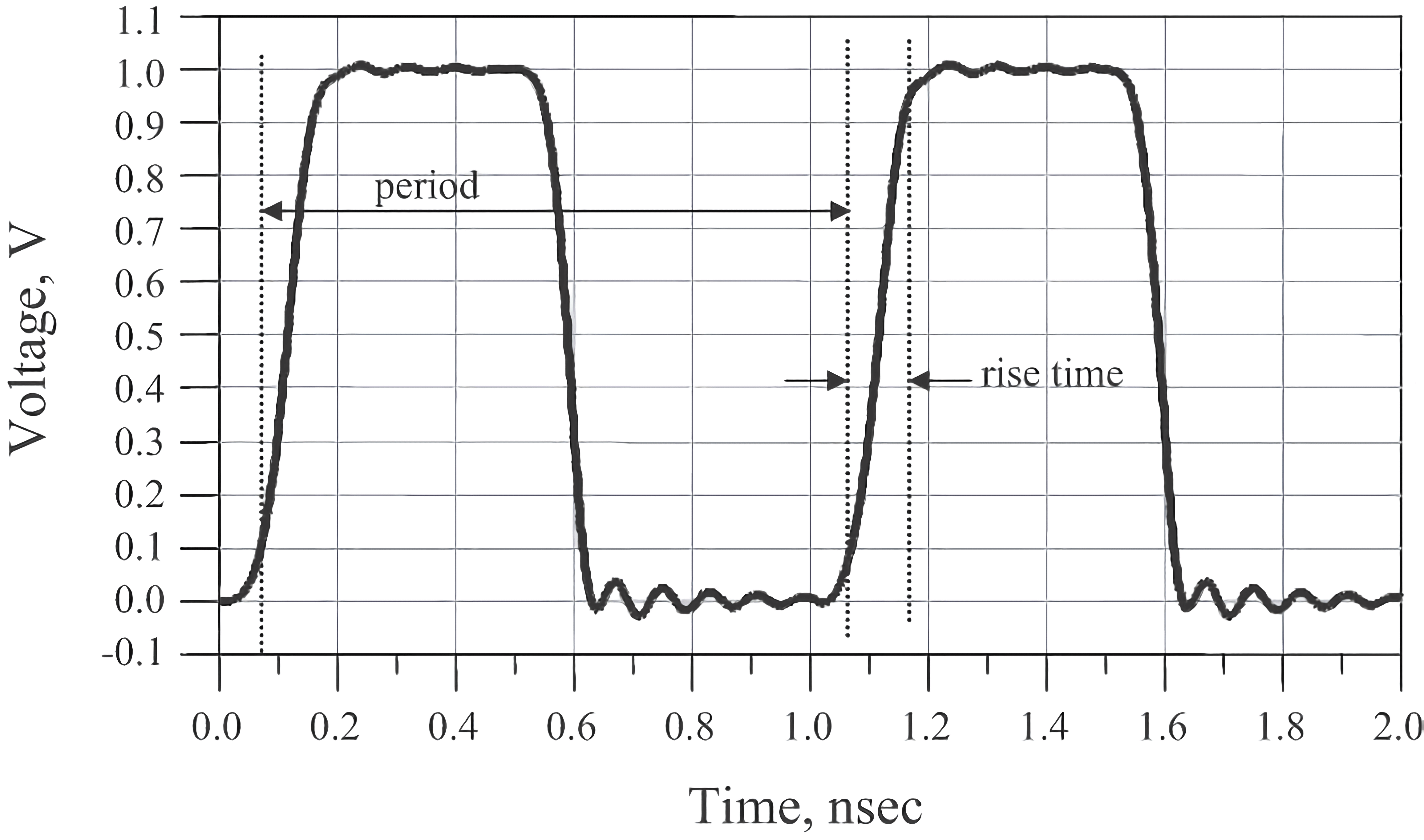
The clock period is the time it takes for the signal to complete one cycle, typically measured in nanoseconds. Clock frequency, on the other hand, is the number of cycles per second, which is the reciprocal of the period. For instance, a signal with a period of 1 ns has a frequency of 0.1 GHz (1/10 ns).

The rising edge is usually defined as the time it takes for the signal to transition from 20% to 80% of its peak amplitude (sometimes defined as 10% to 90%). The falling edge is typically shorter than the rising edge, primarily due to the faster conduction speed of N-MOS compared to P-MOS in typical CMOS structures. This discrepancy between rising and falling edges can lead to signal integrity issues.

Frequency Domain

The frequency domain is a mathematical domain where sinusoidal waves are commonly used. This is because any waveform in the time domain can be synthesized using sinusoidal waves.

The frequency domain offers a more concise way to describe the same information. As shown in the diagram below, on the left, there is a description of a sinusoidal wave in the time domain, which can be completely represented by three parameters: frequency, amplitude, and phase. On the right is the description in the frequency domain, where frequency and amplitude can be represented by a single point (in most cases, phase is omitted):

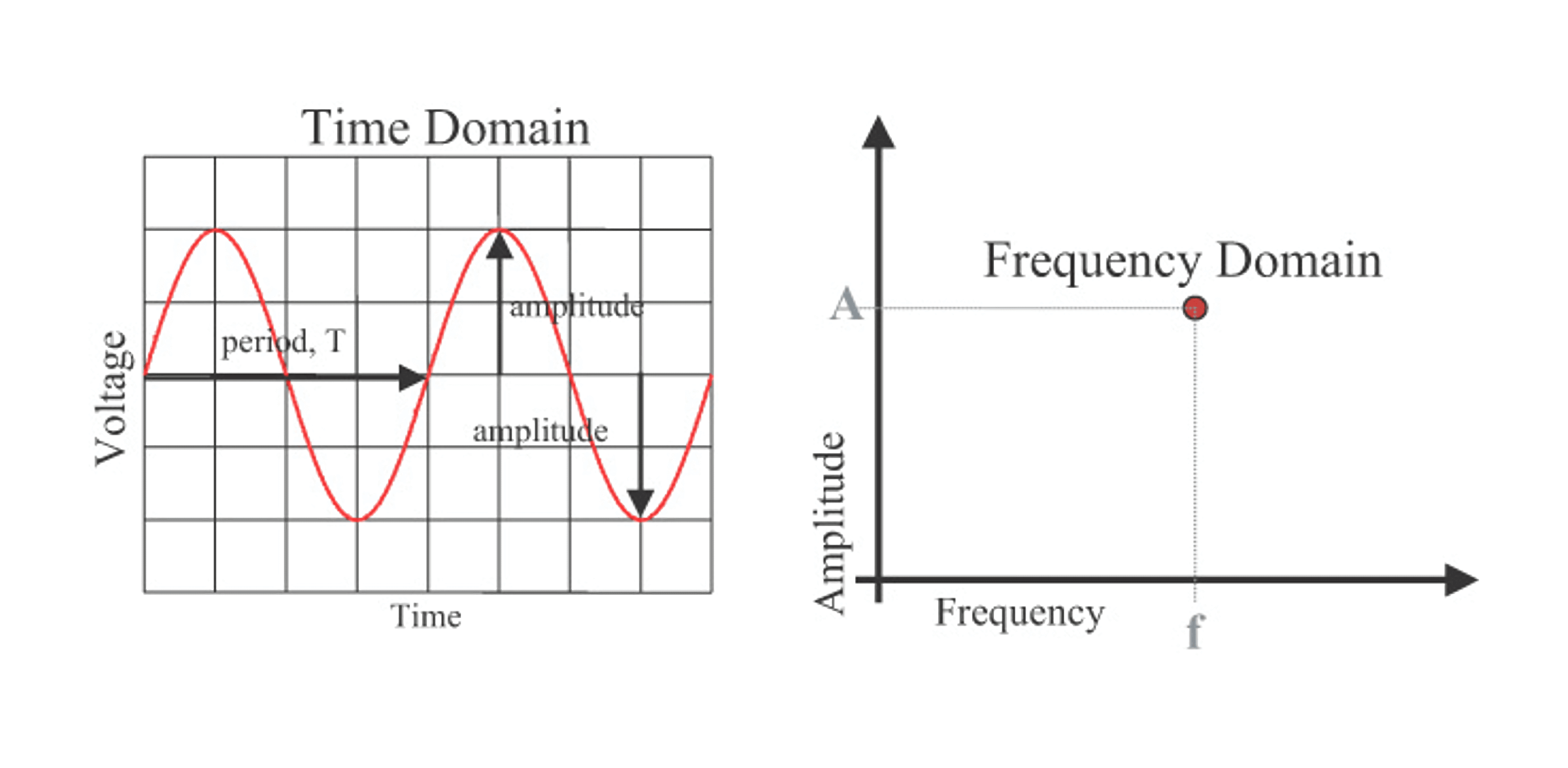
In the frequency domain, representing a sinusoidal wave requires only one point. If there are multiple frequency points, this collection is referred to as a spectrum.

By framing general electrical interconnect issues in the frequency domain and using sinusoidal wave descriptions, it becomes easier to understand and address them.

Transformation from Time Domain to Frequency Domain

To transform from the time domain to the frequency domain, the method used is the Fourier transform. There are three types of Fourier transforms: the Fourier integral (FI), the discrete Fourier transform (DFT), and the fast Fourier transform (FFT).

The Fourier integral is used to transform ideal mathematical expressions from the time domain into a frequency domain representation. It involves integrating over the time axis from negative infinity to positive infinity, resulting in a continuous frequency domain function ranging from zero to positive infinity.

However, in practice, waveforms in the time domain are composed of a series of discrete points. In such cases, the discrete Fourier transform can be used to convert the waveform into the frequency domain (assuming the time domain is periodic). Unlike the Fourier integral, the Fourier transform can be achieved by simple summation.

The fast Fourier transform employs fast matrix algebraic methods and is only applicable when the number of data points in the time domain is a power of 2 (e.g., 256, 512, 1024 points). Depending on the number of data points, the FFT can significantly accelerate the computation compared to the standard discrete Fourier transform.

It's worth noting that the FFT requires the signal to be periodic, so coherent sampling of the original signal or windowing after sampling is necessary.

Transformation from Frequency Domain to Time Domain

The frequency domain contains information about the frequencies and amplitudes of all sinusoidal components in a waveform. To obtain the time domain waveform, you can perform an inverse transformation by multiplying each frequency component by its corresponding time domain sinusoid and summing them together. This process is known as the Fourier inverse transform.

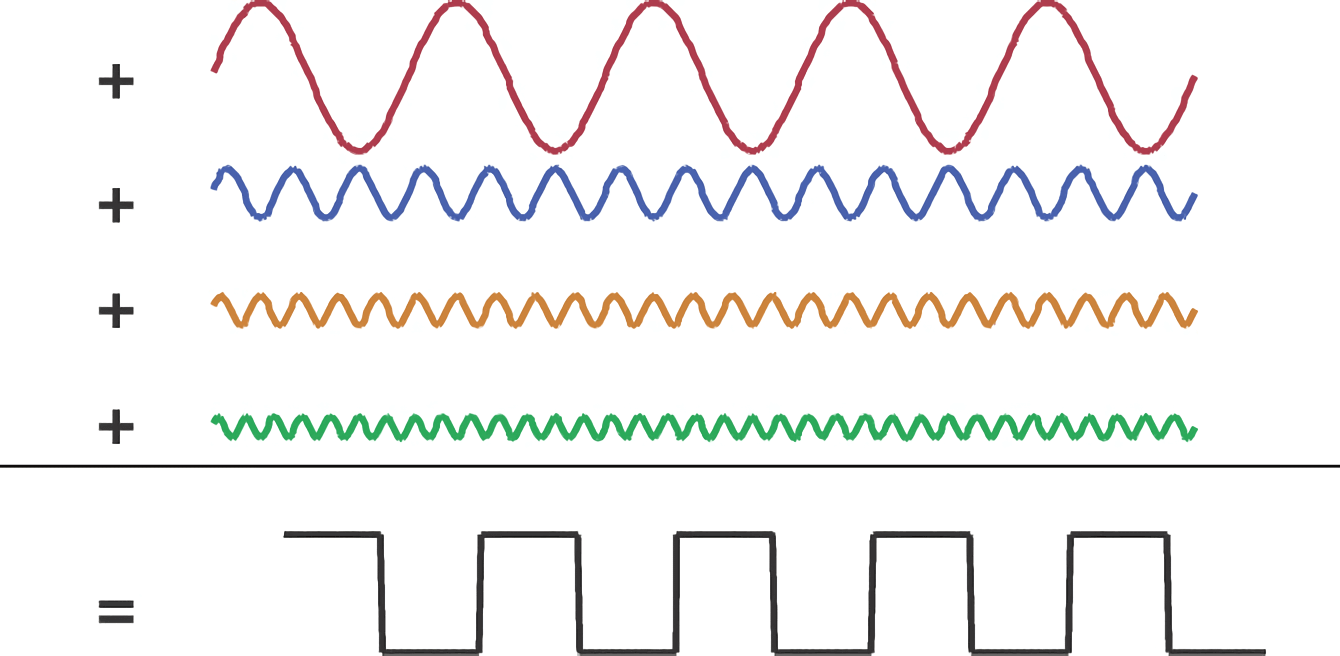
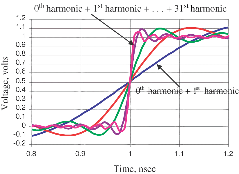
A square wave, for example, is the result of adding multiple harmonics of sinusoidal waves. The more harmonics added, the steeper the rising edge becomes, approaching an ideal square wave:

Bandwidth and Rising Edge

Bandwidth represents the highest effective frequency component in the spectrum (because in digital signals, the lowest frequency is always direct current). It denotes the frequency range in the signal spectrum. The choice of bandwidth directly impacts the shortest rising edge in the time domain waveform. For an ideal square wave, as an example, a wider bandwidth results in a shorter rising edge, making the waveform closer to an ideal square wave.

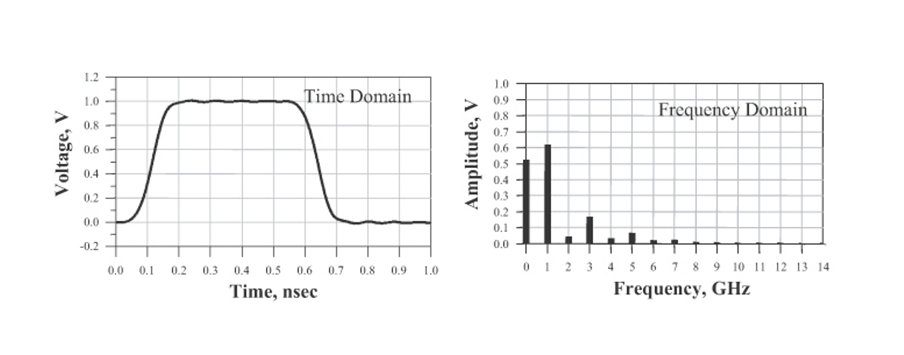
Note that "effective" signifies that the harmonic amplitudes of the signal are above 70% of the corresponding harmonic amplitudes in an ideal square wave of the same fundamental frequency.

For instance, if only the 0th, 1st, and 3rd harmonics are used to synthesize the time domain waveform, the waveform's bandwidth is determined by the 3rd harmonic, which is 3 GHz.

According to the empirical rule derived from experiments, the relationship between bandwidth and the rise time is given by \(BW=\frac{0.35}{RT}\), where BW represents the bandwidth in gigahertz (GHz) and RT stands for the 10%-90% rise time in nanoseconds (ns). For example, if the rise time of a signal is 0.1 ns, then the signal's bandwidth is 0.35 GHz, and vice versa. (Note the corresponding units: GHz corresponds to ns, MHz corresponds to microseconds (us)).

References and Acknowledgments

• "Signal Integrity and Power Integrity Analysis"
• Illustrated Fourier Series & Fourier Transform
• Fundamentals of Fourier Transform Series

Original: https://wiki-power.com/
This post is protected by CC BY-NC-SA 4.0 agreement, should be reproduced with attribution.

This post is translated using ChatGPT, please feedback if any omissions.